07-22-2022

Making the Famous Magic Wand 33x Faster

Intro

This case is a remake of a well-known “magic wand” experiment. Last year, Pete Warden, the famous creator of the TensorFlow Lite for Microcontrollers (TFLM) framework, ran a workshop on building a digital ML-based magic wand at the tinyML Summit. Today, it’s one of the most popular gesture recognition experiments as only on Hackster.io, dozens of “magic wand” tutorials can be found.

Can I build a model better than Pete Warden? It turned out that today everyone can do it. Only a year ago, the solution offered by Pete Warden seemed to be a breakthrough, but now it’s no longer small, fast, and accurate enough. Thanks to the new technology, now I can show how you can build a similar model automatically, and with impressive results.

For my experiment, I used an original TFLM model built into the Arduino SDK, and also collected my own dataset to build a new model on Neuton.AI. As the hardware component, I used Arduino Nano 33 BLE Sense, as in the original experiment.

Competing with TensorFlow Lite for Microcontrollers

Using the public magic wand dataset

For my first experiment, I used an official TensorFlow Lite MagicWand example.

The trained TensorFlow Lite model is built into the Arduino SDK and is described in the official Google documentation.
The dataset is provided in the official TensorFlow repository.

For benchmarking, I used the trained TFLM model from the Arduino SDK and trained a Neuton model using the dataset in the mentioned repository.

Both models are validated on the same hold-out dataset and were tested on the same MCU (Arduino Nano 33 BLE Sense).

Please find the model codes attached:

Neuton model on TensorFlow example data (Arduino sketch)
TensorFlow trained model (Arduino sketch)

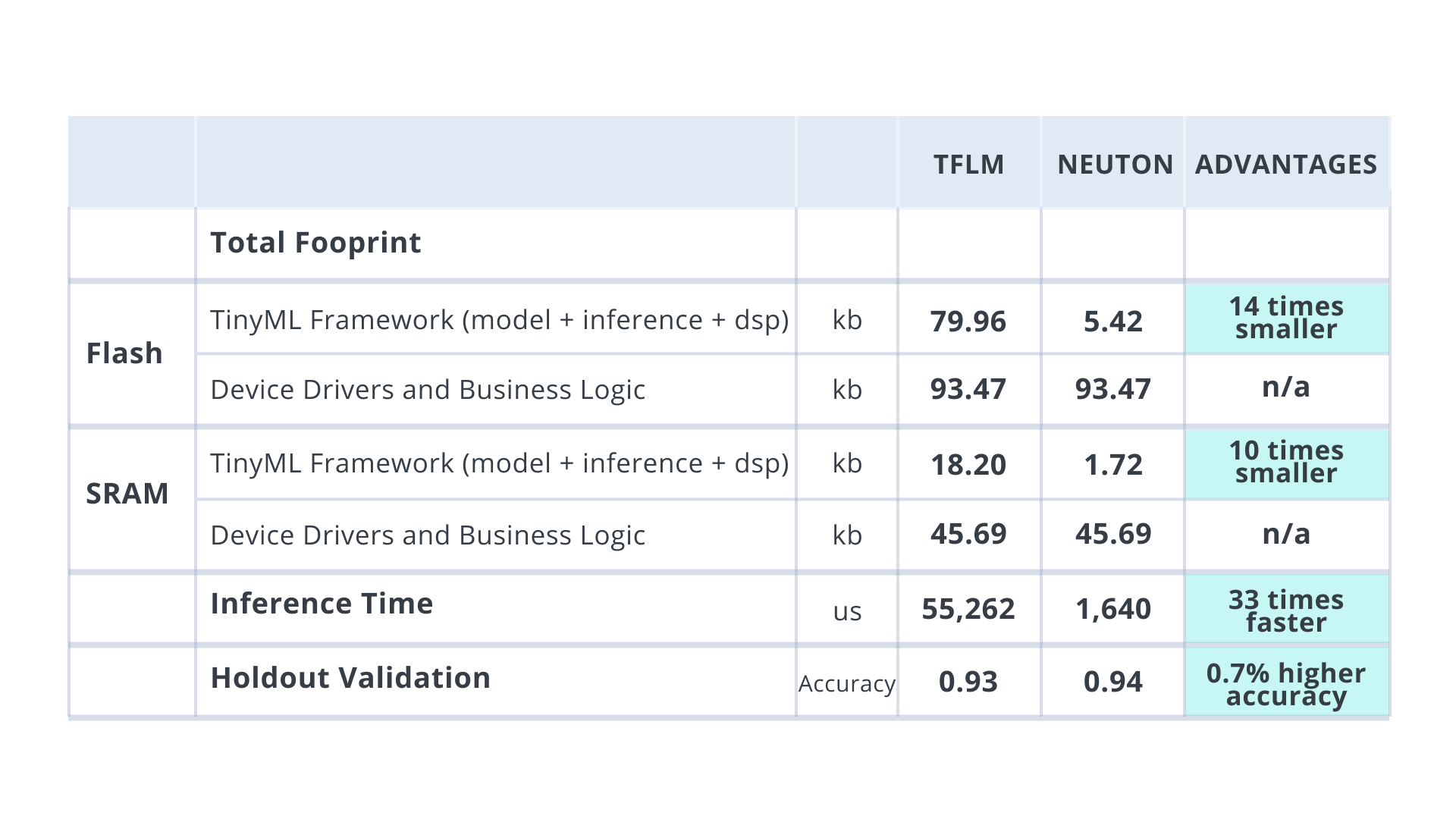
In the table below, you can see the resulting benchmarks. Models built with Neuton have advantages in several if not all aspects: accuracy, size, inference time, and most importantly, they are built automatically, hence also accelerating the time to market. Additionally, TensorFlow Lite for Microcontrollers (TFLM) and Neuton solutions were embedded into Arduino Nano 33 BLE Sense (CortexM4).

RESULTING BENCHMARKS

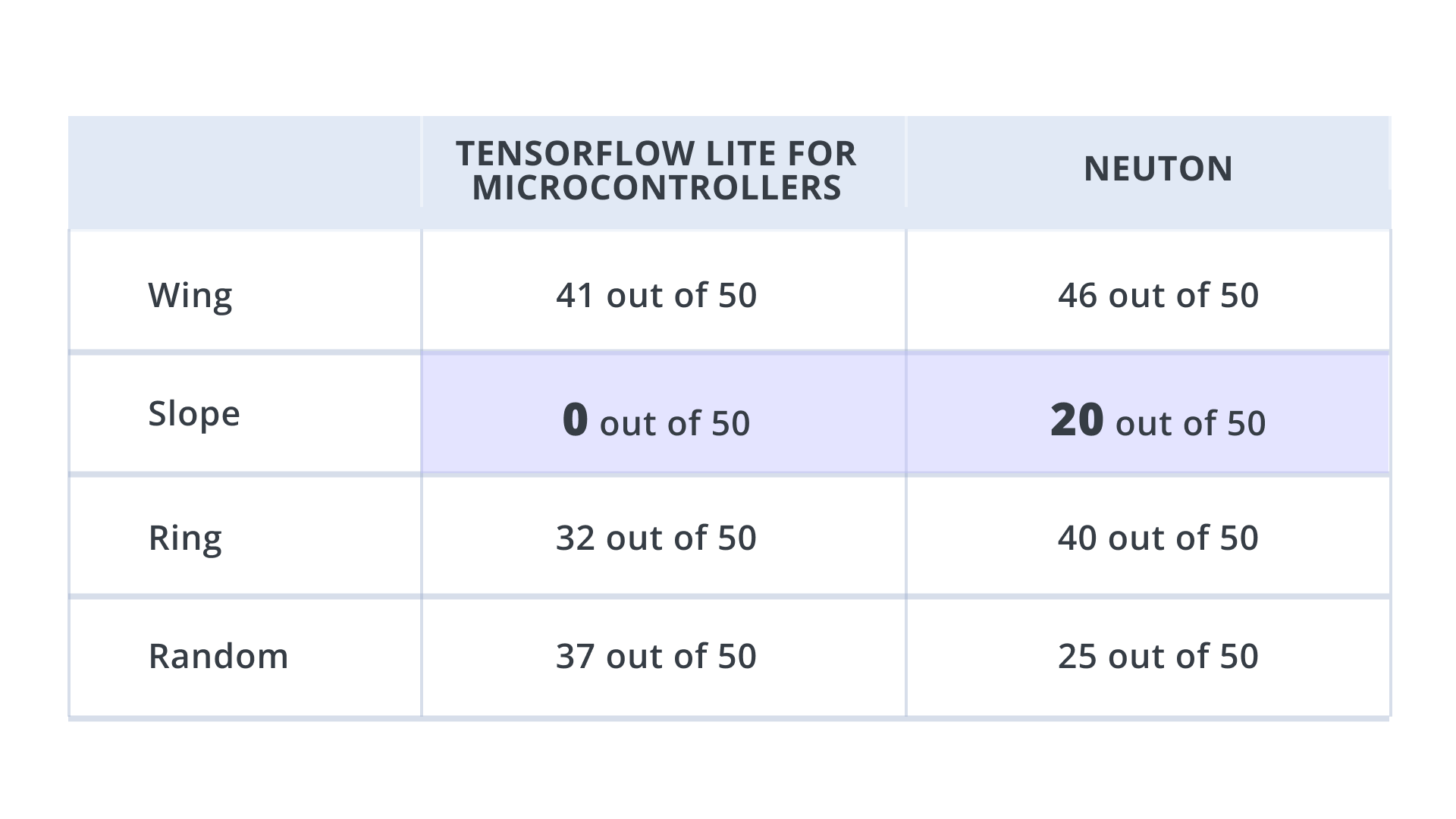
TensorFlow’s model was capable of recognizing only 3 classes: Wing, Ring, and Random, but it was not capable of recognizing Slope. On the other hand, Neuton successfully recognized all 4 classes. Below you can see the results of the experiments.

NUMBER OF CORRECTLY RECOGNIZED CLASSES

Collecting my own magic wand dataset

I decided to reproduce this experiment from the very beginning, namely from the data collection stage since in the previous experiment with the TF dataset, I could not control the data collection. The aim was to prove that the real-time accuracy on the device could be improved. I have used the Arduino Nano 33 BLE Sense for this experiment as well.

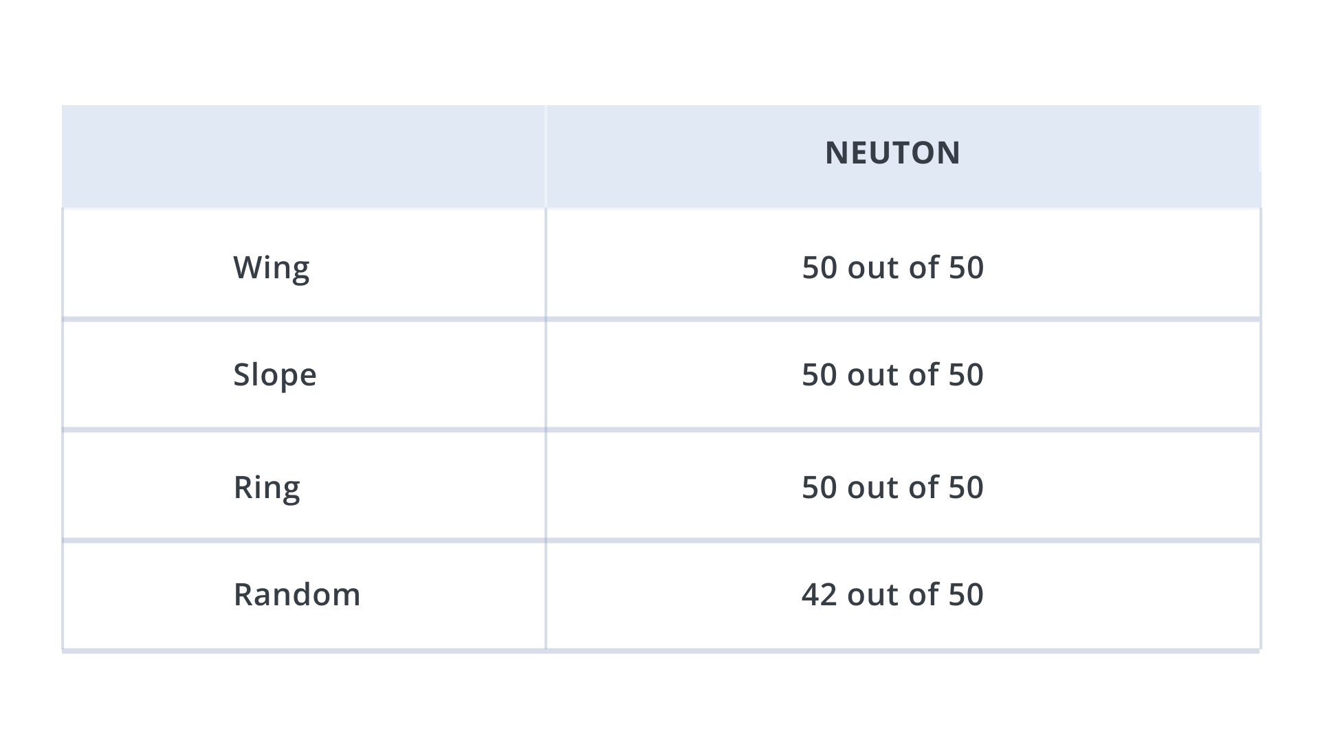
After training the Neuton model on the data I collected, I recorded the following real-time outcomes which showed great improvement in accuracy:

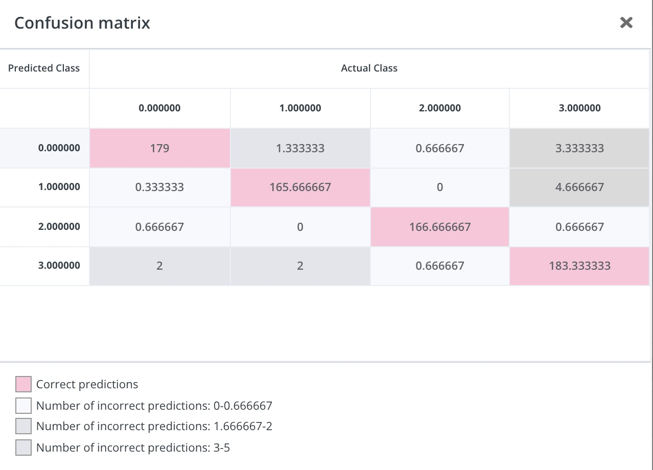
NUMBER OF CORRECTLY RECOGNIZED CLASSES IN MY OWN MAGIC WAND DATASET

Procedure

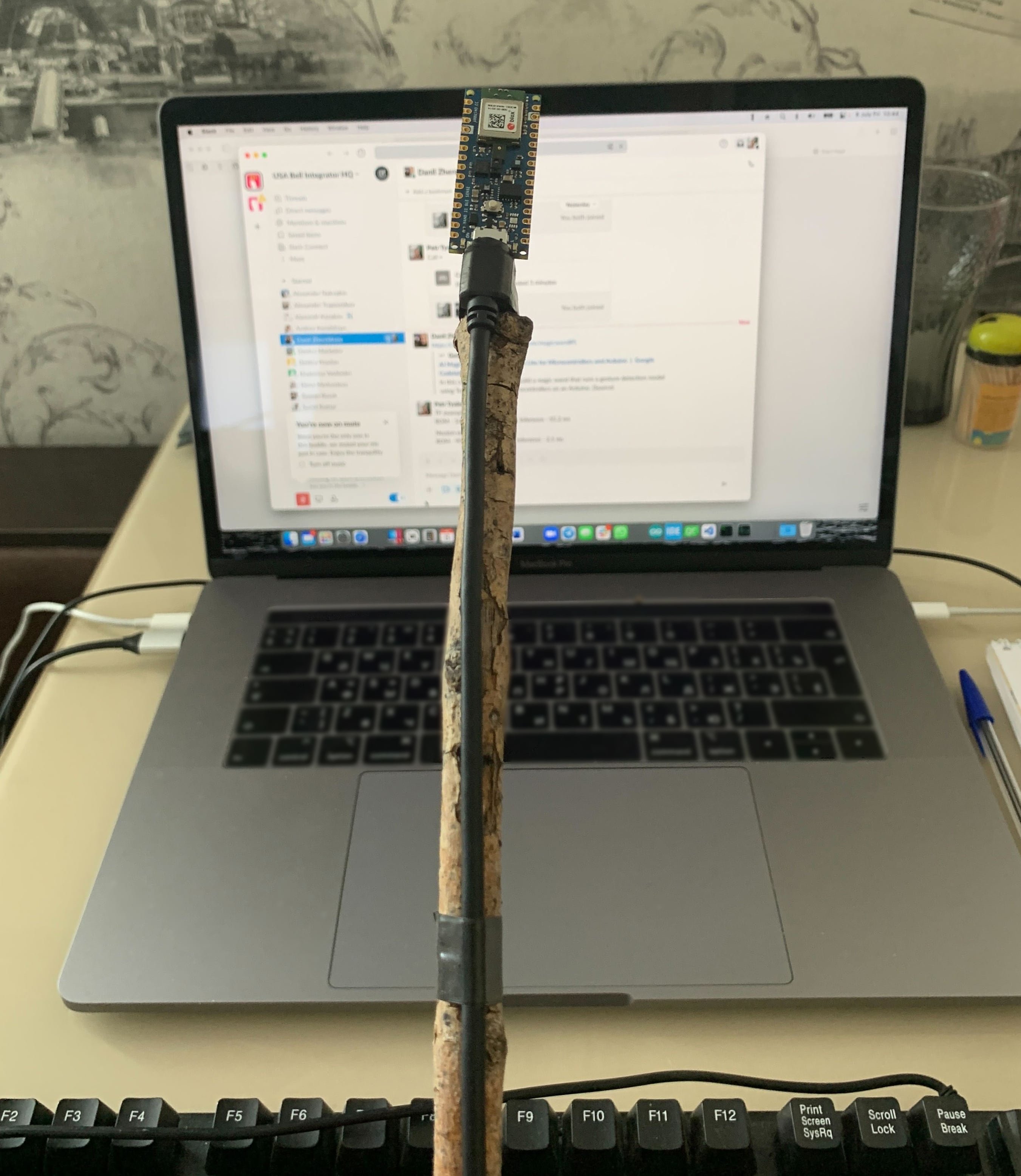
The onboard accelerometer is the main sensor for this use case. The board is attached to the end of a stick/wand with a USB facing downwards, towards the place where you hold it so that the cable runs down the handle. Use sticky tape, a velcro strap, or some easy-to-remove method to attach the board and cable to the wand.

Step 1: Data Collection

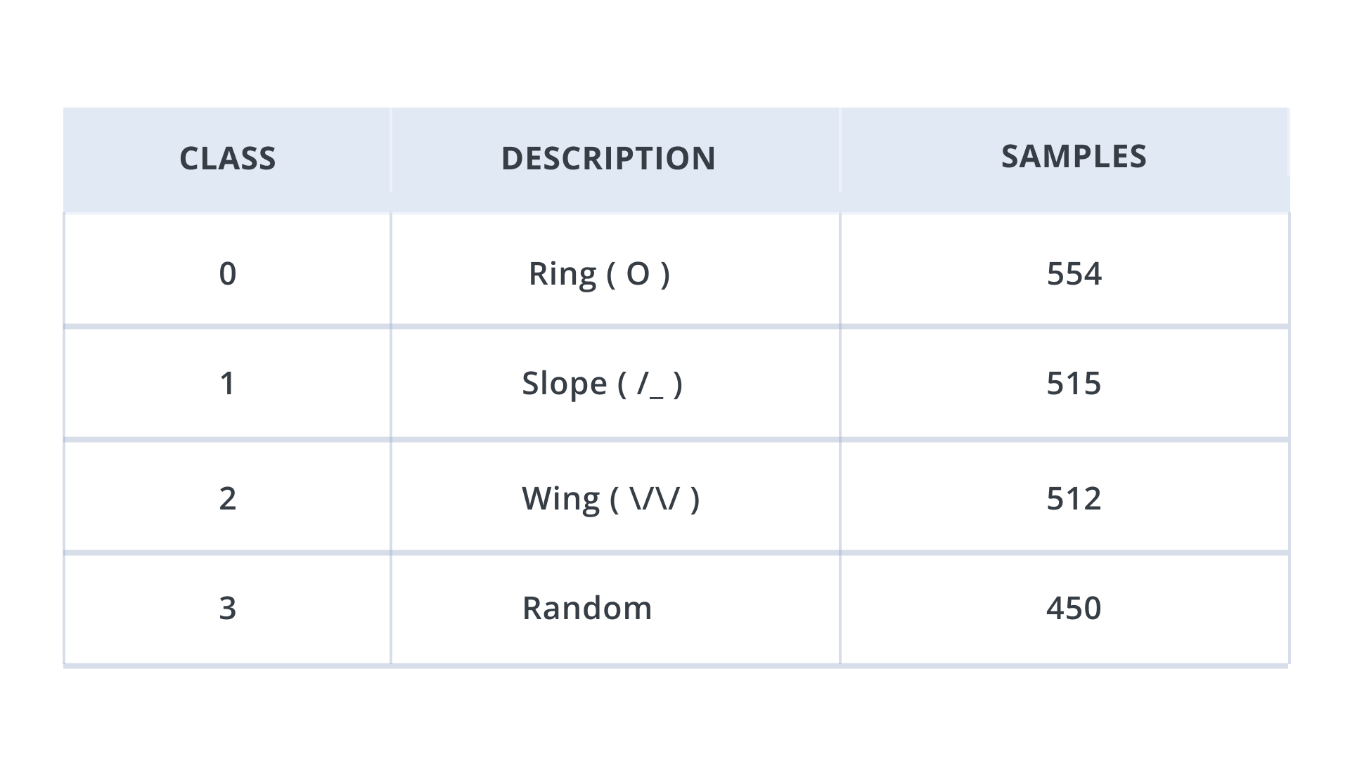
The data collection included four classes: Wing, Slope, Ring, and Random class. Sensors reading were collected at 100 Hz frequency, with a sample duration of 2 seconds. So you get 200 rows of accelerometer sensor data for each sample. Check the instruction on how to perform the motion activity for each gesture.

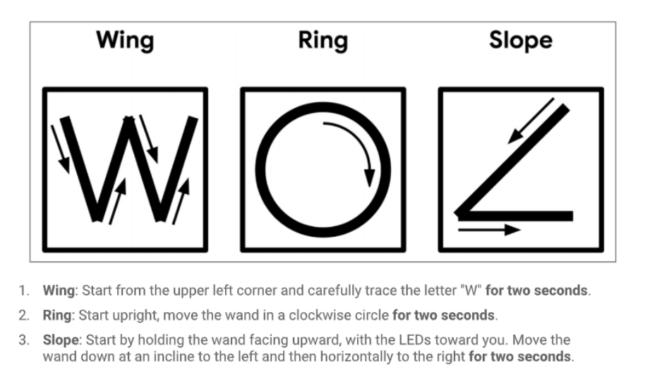
Any other gestures apart from the above are treated as a random class. The instruction for data collection, codes and datasets can be found here:

Data collection explanatory document
Codes for data collection
Data that I have collected

Below is the summary of the collected training dataset.

TRAINING DATASET

In a similar way, collect validation dataset as well.

Step 2: Model Training

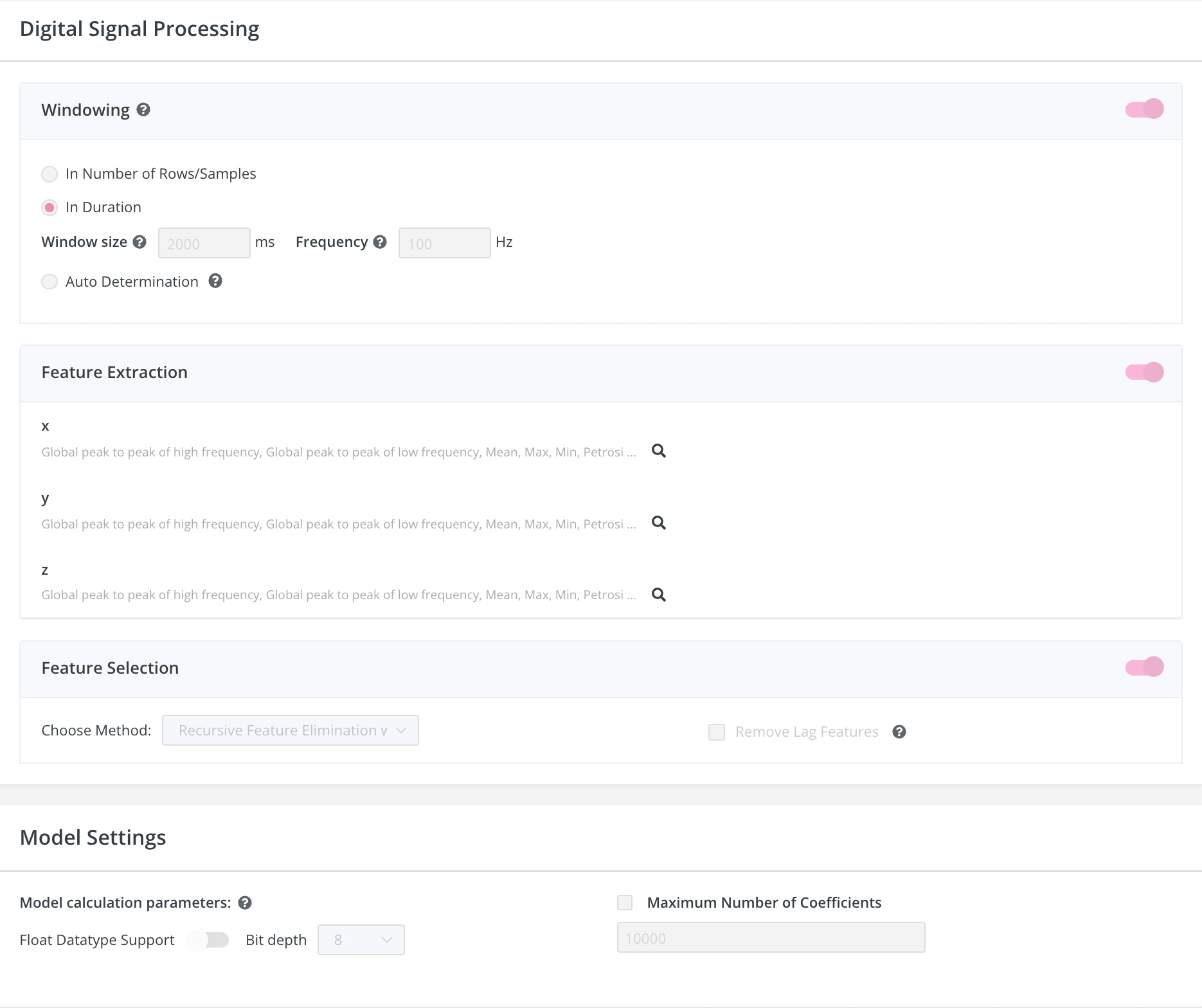
Upload your dataset on the Neuton platform and enable the following training settings:

Input data type: FLOAT32

Normalization type: Unified Scale for All Features

Window size: 2000ms

Frequency: 100 Hz

Feature Extraction Method: Digital Signal Preprocessing Neuton pipeline (enabled by default) which creates statistical features for each of the original features processing a window of 2000ms.

Feature Selection Method:

Disable the option Remove Lag Features
Select Recursive Feature Elimination with Cross-validation

Bit depth: 8-bit

Once training is complete, you can check the metrics on the console. In my case, I got Accuracy: 0.977028.

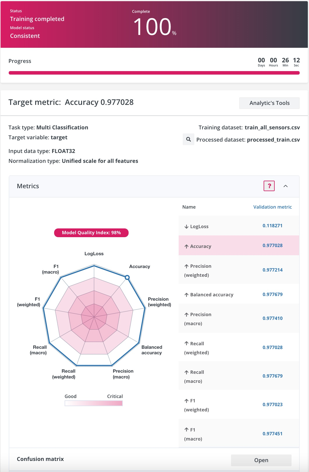
From the confusion table, I can see that the model works really well across all target classes.

I got a model that weighs about 1 kb!

Please find the Neuton model on the data I have collected.

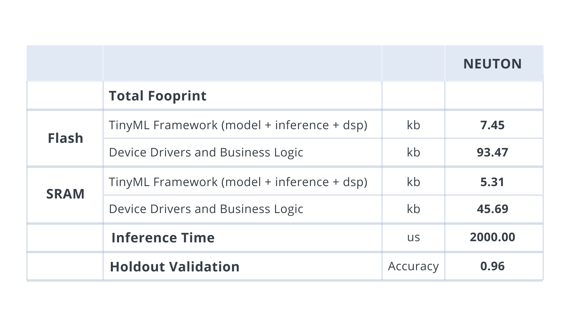
The total footprint of the solution embedded into the MCU is highlighted in the table below:

Step 3: Model Embedding and Inference

In this final step, I am going to embed the model to the device. Download your model as a Zip archive from the Neuton platform. Extract all the downloaded files and put them inside a folder named “src” in your project directory. It should look as shown below:

C:.
|   .DS_Store
|   MagicWandTestPP.ino
|
\---src
    |   .DS_Store
    |   neuton.c
    |   neuton.h
    |   README.md
    |
    +---converted_models
    |       README.md
    |
    +---fe
    |   \---statistical
    |       |   Common.c
    |       |   Common.h
    |       |   DSP.h
    |       |   DSPF32.c
    |       |   DSPF32.h
    |       |
    |       \---fht
    |               fhtf32.c
    |               fhtf32.h
    |
    +---model
    |       dsp_config.h
    |       model.h
    |
    +---postprocessing
    |   \---blocks
    |       \---moving_average
    |               moving_average.c
    |               moving_average.h
    |
    +---preprocessing
    |   |   .DS_Store
    |   |
    |   \---blocks
    |       |   .DS_Store
    |       |
    |       +---normalize
    |       |       normalize.c
    |       |       normalize.h
    |       |
    |       \---timeseries
    |               timeseries.c
    |               timeseries.h
    |
    \---target_values
            multi_target_dict_csv.csv

To understand how the model will be functioning on the device, we will have a look at some important functions in the Arduino codes.

In the function, void OnDataReady(void *ctx, void *data), we pass the data buffer which contains the accelerometer sensor values for the defined window size using the callback neuton_model_window_size(). In this experiment, the window size is 2 seconds which means 200 rows of accelerometer data or 600 values of x, y and z acceleration axis to be fed into the neuton_model_set_inputs(inputs).

void OnDataReady(void *ctx, void *data)
{
  input_t *inputs = (input_t*)data;
  size_t inputsCount = neuton_model_inputs_count();
  size_t windowSize = neuton_model_window_size();

  for (size_t i = 0; i < windowSize; i++)
  {
#ifndef NO_CALC
    if (neuton_model_set_inputs(inputs) == 0)
    {
      float* outputs;
      uint16_t index;
      uint64_t start_time = micros();
      if (neuton_model_run_inference(&index, &outputs) == 0)
      {

        uint64_t stop_time = micros();

After the neuton_model_run_inference(&index, &outputs) callback is invoked, the model returns the output predictions. We use a custom function called NeutonPostprocessingBlockMovingAverageProcess(&avg, outputs, &outputs, &index) to accept probabilities from the neural network, average these probabilities, and return averaged probabilities if one class reaches a threshold (we have set a threshold to 0.95f). Also, if no gesture is recognized (index 3), we cancel suppression.

if (NeutonPostprocessingBlockMovingAverageProcess(&avg, outputs, &outputs, &index) == 0)
        {
          if (index == 0)
          {
            Serial.print(" Ring: O      ");
          }
          if (index == 1)
          {
            Serial.print("Slope: /_     ");
          }
          if (index == 2)
          {
            Serial.print(" Wing: \\/\\/   ");
          }
          if (index == 3)
          {
//             Serial.print("Ooops! Nothing");
            avg.suppressionCurrentCounter = 0;
            continue;
          }

          Serial.print("     score: ");
          Serial.println(outputs[index], 2);
        }
      }
    }
#endif

    inputs += inputsCount;
  }

Conclusion

This remake of a popular case vividly demonstrates that a magic wand can be several times faster, smaller and more accurate than in the original experiment. The use of Neuton empowers the model to have better results on such ML applications. It's amazing how quickly the TinyML technology develops. A year ago, such experiments seemed pure magic, but now any schoolboy can produce similar solutions automatically.

Are you inspired to create your own project? Try Neuton for free right now!